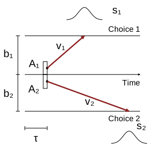
Quick start

Installation

pyLBA requires Python 3.10 or newer. Install from the repository:

pip install git+https://github.com/rgs2151/pyLBA.git

Simulation

Create a model and specify the starting-point bound, thresholds, drift parameters, and non-decision time:

from pyLBA import LBAModel, LBAParameters

model = LBAModel()
parameters = LBAParameters(
    A=1.0,
    b=[2.0, 3.0],
    v=2.0,
    s=1.0,
    tau=0.1,
)
data = model.generate_data(500, parameters, seed=42)
print(data.head())

A scalar is shared across accumulators. A vector supplies one value per accumulator. The number of accumulators is inferred from parameter vectors; pass n_acc explicitly when all parameters are scalar.

The result is a pandas DataFrame with response times in rt and zero-based choice labels in response. A fixed seed reproduces the simulated data.

Fitting and prediction

This example estimates thresholds while holding the other parameters fixed:

model.fit_mcmc(
    data,
    priors={"A": 1.0, "v": 2.0, "s": 1.0, "tau": 0.1},
    draws=1000,
    tune=1000,
    chains=4,
    random_seed=42,
)
predictions = model.predict(100, seed=7)

import arviz as az
print(az.summary(model.trace, var_names=["b"]))
print(model.parameters)

trace contains the posterior samples. parameters contains posterior means, and predict simulates at those means. See Bayesian fitting for default priors and custom distributions.

Plot simulated data

import matplotlib.pyplot as plt

for response, trials in data.groupby("response"):
    plt.hist(trials.rt, bins=30, alpha=0.5, label=f"Response {response}")
plt.xlabel("Response time")
plt.ylabel("Trials")
plt.legend()
plt.show()