Examples

Two-choice simulation

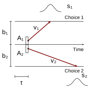
Specify a vector when a parameter differs between choices. Here, both choices share a non-decision time, while their starting ranges, thresholds, and drift means differ:

from pyLBA import LBAModel, LBAParameters

model = LBAModel()
parameters = LBAParameters(
    A=[0.4, 0.3],
    b=[1.5, 1.05],
    v=[2.8, 1.8],
    s=0.45,
    tau=0.16,
)
data = model.generate_data(1000, parameters, seed=42)
print(data.groupby("response").rt.agg(["count", "mean", "median"]))

The response labels are 0 and 1. Drift is sampled once per accumulator per trial, then remains constant until a threshold is reached.

Five-choice simulation

The same interface supports races with more alternatives:

parameters = LBAParameters(
    A=0.5,
    b=[1.5, 1.6, 1.7, 1.8, 1.9],
    v=[2.5, 2.3, 2.1, 1.9, 1.7],
    s=0.6,
    tau=0.2,
)
data = model.generate_data(2000, parameters, seed=7)
choice_counts = data.response.value_counts().reindex(range(5), fill_value=0)
print(choice_counts)

For identical parameters across alternatives, supply n_acc explicitly:

shared = LBAParameters(A=0.5, b=1.5, v=2.0, s=0.6, tau=0.2)
balanced = model.generate_data(1000, shared, n_acc=5, seed=7)

Fit recorded responses

A CSV file needs rt and response columns. Response times must be positive and finite, and responses must be non-negative integers numbered from zero. Convert time units before fitting; tau uses the same units as rt.

import pandas as pd
import arviz as az

observed = pd.read_csv("responses.csv", usecols=["rt", "response"])
model.fit_mcmc(
    observed,
    n_acc=2,
    draws=1000,
    tune=1000,
    chains=4,
    cores=4,
    random_seed=42,
)
print(az.summary(model.trace, var_names=["A", "b", "v", "tau"]))
model.trace.to_netcdf("posterior.nc")

Set n_acc to the number of possible choices, including alternatives with no observed responses. On systems that restrict worker processes, use cores=1. The Bayesian fitting guide explains the default priors and fixed-parameter fits.

Compare fitted predictions with observations

predict simulates at posterior mean parameters. Compare the resulting choice frequencies and response times with the observed data:

predictions = model.predict(len(observed), seed=8)
frequencies = pd.DataFrame({
    "observed": observed.response.value_counts(normalize=True),
    "predicted": predictions.response.value_counts(normalize=True),
}).fillna(0).sort_index()
print(frequencies)

import matplotlib.pyplot as plt

fig, ax = plt.subplots()
ax.hist(observed.rt, bins=30, density=True, histtype="step", label="Observed")
ax.hist(predictions.rt, bins=30, density=True, histtype="step", label="Predicted")
ax.set(xlabel="Response time", ylabel="Density")
ax.legend()
plt.show()

These predictions do not integrate over posterior uncertainty. Inspect the posterior samples before interpreting a fitted model.

Notebook

Download the complete example notebook for a three-choice simulation, visualization, threshold fit, and prediction.