Bayesian fitting#
Fit with PyMC#
fit_mcmc constructs a PyMC model and samples the posterior using the joint
response-time and choice likelihood. Sampling options such as target_accept
and random_seed are forwarded to pymc.sample.
model.fit_mcmc(
    data, n_acc=2,
    draws=1000, tune=1000, chains=4,
    target_accept=0.9, random_seed=42,
)
Default priors#
Each accumulator receives these defaults:
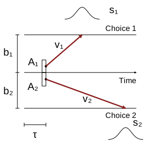
A: HalfNormal with standard deviation 2.b:A + b_gap, with a HalfNormal(2) prior onb_gap.v: Normal with mean 2 and standard deviation 1.s: fixed at 1 to define the evidence scale.tau: Uniform between zero and the shortest observed response time.
The threshold parameterization ensures b > A. The bound on tau keeps
the default prior within observed response-time support. Fixing s removes
the scale ambiguity: multiplying A, b, v, and s by the same
positive factor leaves decision times unchanged.
Custom priors and fixed parameters#
The priors dictionary accepts fixed numbers or vectors, or callables
with arguments (name, n_acc). Callables create PyMC variables inside the
fitting model:
import pymc as pm

priors = {
    "A": 1.0,
    "v": lambda name, n_acc: pm.Normal(
        name, mu=2, sigma=0.5, shape=n_acc
    ),
    "s": 1.0,
    "tau": 0.1,
}
model.fit_mcmc(data, priors=priors, random_seed=42)
Omitted parameters use their defaults. If A is overridden and b is not,
the default threshold remains A + b_gap. Custom distributions must respect
the parameter domains; if s is estimated, constrain another parameter to
set the evidence scale. At least one parameter must remain free for sampling.
Posterior summaries and predictions#
import arviz as az

summary = az.summary(model.trace, var_names=["b", "v"])
az.plot_trace(model.trace, var_names=["b", "v"])
predictions = model.predict(500, seed=42)
model.trace is ArviZ InferenceData. model.parameters contains the
posterior means, including fixed parameters. predict simulates using
those means; it does not integrate over posterior parameter uncertainty.
EM#
EM fitting is not implemented. fit_em raises NotImplementedError.