
CNN: MNIST Classification#
Four convolutional stages learn local stroke features from handwritten digits. The run uses 55,000 training images, a seeded 5,000-image validation split, and all 10,000 official test images.
The outputs below are saved from local GPU training. Documentation builds render these saved outputs without running cells.
JAXsaw 0.1.0 · JAX 0.5.3
[CudaDevice(id=0)]
Architecture#
Input [B,1,28,28] in [0,1]; output [B,10] logits. The input is zero-padded to 32×32. Four convolution–ReLU–max-pooling stages reduce the spatial grid to 16×16, 8×8, 4×4, and 2×2, with 16, 32, 64, and 128 channels. Training dropout consumes an explicit runtime stream. Evaluation disables dropout.
The definition below is the actual package implementation used by this run.
class DigitCNN(nn.Module):
    """Four convolution/pooling stages for MNIST NCHW images.

    Zero padding expands 28x28 to 32x32 before four reductions to 16, 8,
    4, and 2 pixels per side. Earlier two-stage checkpoints are incompatible.
    """

    def __init__(self, width=16, classes=10, *, rngs):
        super().__init__()
        self.conv1 = nn.Conv2d(1, width, 3, padding=1, rngs=rngs)
        self.conv2 = nn.Conv2d(width, width * 2, 3, padding=1, rngs=rngs)
        self.conv3 = nn.Conv2d(width * 2, width * 4, 3, padding=1, rngs=rngs)
        self.conv4 = nn.Conv2d(width * 4, width * 8, 3, padding=1, rngs=rngs)
        self.pool = nn.MaxPool2d(2, stride=2)
        self.dropout = nn.Dropout(0.2)
        self.head = nn.Linear(width * 8 * 2 * 2, classes, rngs=rngs)

    def forward(self, x, *, rngs=None):
        x = jnp.pad(x, ((0, 0), (0, 0), (2, 2), (2, 2)))
        for conv in (self.conv1, self.conv2, self.conv3, self.conv4):
            x = self.pool(F.relu(conv(x)))
        return self.head(self.dropout(x.reshape(x.shape[0], -1), rngs=rngs))
Objective and optimization#
Training uses an explicit step. Data iteration, evaluation, and artifact writing remain outside compiled computation.
@jit
def cnn_step(model, optimizer, batch, rngs):
    x, y = batch

    def objective(candidate):
        logits = candidate(x, rngs=rngs)
        return F.cross_entropy(logits, y), (logits.argmax(-1) == y).sum()

    (loss, correct), grads = value_and_grad(objective, has_aux=True)(model)
    optimizer.step(grads)
    return {"loss": loss, "correct": correct, "count": y.size}
Reproduce the run#
Select one GPU before launching Python or Jupyter: CUDA_VISIBLE_DEVICES=0. The recipe below creates a new run directory and does not overwrite completed results. Leave TRAIN=False to inspect an existing local run. Checkpoints are gitignored; this notebook retains the figures and metrics for publication.
from examples.train_gallery import RECIPES
import subprocess
TRAIN = False
command = [sys.executable, '-m', 'examples.run', 'cnn', '--download',
           '--output', str(RUN), *RECIPES['cnn']]
print(' '.join(part.replace(str(ROOT) + '/', '')
               for part in ['python', *command[1:]]))
if TRAIN:
    subprocess.run(command,cwd=ROOT,check=True)
if not (RUN / 'report.json').exists():
    raise FileNotFoundError('Run the recipe locally before refreshing notebook outputs.')
report = json.loads((RUN / 'report.json').read_text())
configuration = report['config']
display(pd.DataFrame([{'epochs':configuration['epochs'], 'batch_size':configuration['batch_size'],
                      'seed':configuration['seed'], 'training_examples':report['train_samples'],
                      'validation_examples':report['validation_samples'],
                      'test_examples':report['test_samples']}]))
print('Training device:',', '.join(report['devices']))
python -m examples.run cnn --download --output runs/gallery-four-layer/cnn --epochs 10 --limit 55000 --eval-limit 10000 --batch-size 128
Training device: cuda:0 NVIDIA GeForce RTX 5090
| epochs | batch_size | seed | training_examples | validation_examples | test_examples | |
|---|---|---|---|---|---|---|
| 0 | 10 | 128 | 0 | 55000 | 5000 | 10000 |
Training history#
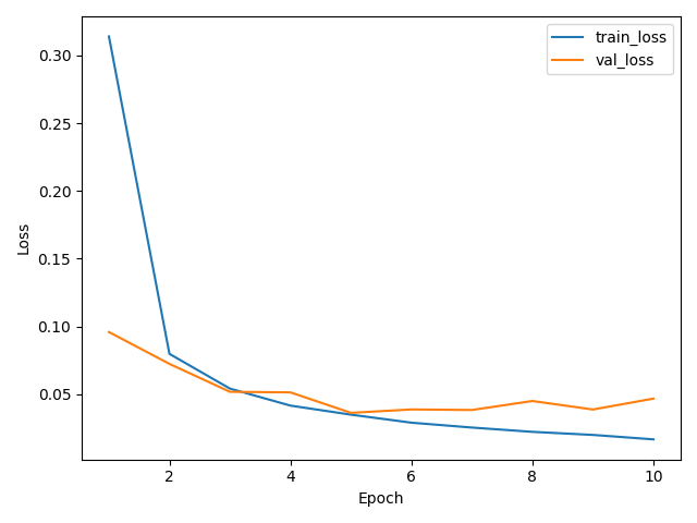
The figure reports actual epoch metrics. For supervised tasks, the checkpoint with the lowest validation loss is selected before test evaluation.
display(Image(filename=str(RUN / 'learning.png')))
if 'val_loss' in report['history'][0]:
    best_epoch = 1 + int(np.argmin([row['val_loss'] for row in report['history']]))
    print('Selected epoch:',best_epoch)
Selected epoch: 5
Evaluation#
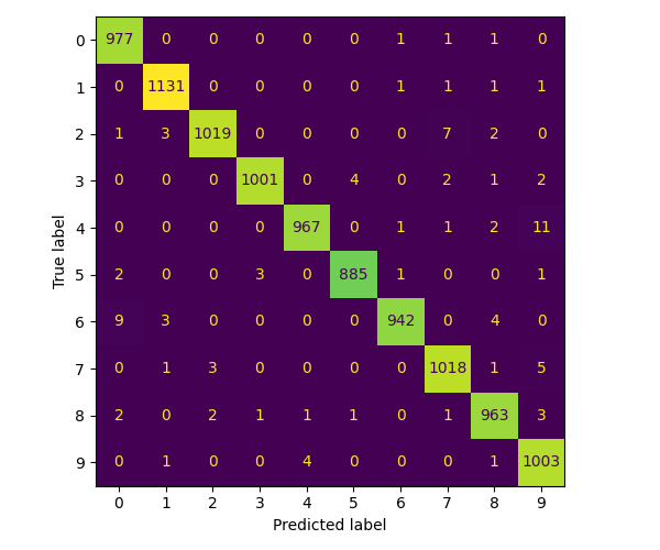
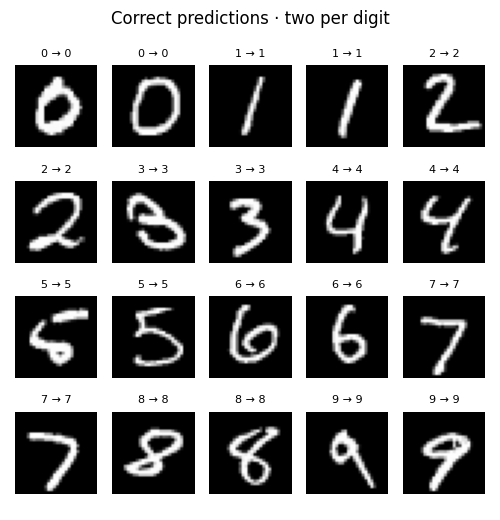
The confusion matrix summarizes all 10,000 official test images. Start with correctly classified examples to see the digit shapes the CNN recognizes, then examine its errors.
metrics = {name:value for name,value in report.items()
           if name in ('test_loss','test_accuracy','majority_baseline_accuracy',
                       'persistence_baseline_mse','perplexity','test_auc','test_brier')}
if metrics:
    display(pd.DataFrame(list(metrics.items()),columns=['Metric','Value']))
print('Timed training loop (including validation/checkpoint work):',round(report['training_seconds'],2),'seconds')
| Metric | Value | |
|---|---|---|
| 0 | test_loss | 0.026346 |
| 1 | test_accuracy | 0.990600 |
| 2 | majority_baseline_accuracy | 0.113500 |
Timed training loop (including validation/checkpoint work): 10.92 seconds
from examples import datasets, plots
_, (test_images, test_labels) = datasets.images(cache=ROOT / 'data')
with np.load(RUN / 'predictions.npz', allow_pickle=False) as saved:
    probabilities, targets = saved['probabilities'], saved['targets']
np.testing.assert_array_equal(test_labels[:len(targets)], targets)
plots.classification(targets, probabilities, RUN / 'classification.png')
plots.digit_gallery(test_images[:len(targets)], targets, probabilities, RUN)
display(Image(filename=str(RUN / 'classification.png')))
Successful predictions#
These are the first two correctly classified test examples for each digit, in dataset order. Labels show true → predicted. The gallery illustrates the learned classes; the full-test accuracy above measures overall performance.
display(Image(filename=str(RUN / 'successes.png')))
Failure analysis#
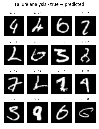
The following grid contains the first sixteen mistakes in test-set order. These examples help identify ambiguous strokes and confusable classes. Their concentration here is deliberate: the full test result is 99.06% accuracy, or 94 errors among 10,000 images.
display(Image(filename=str(RUN / 'mistakes.png')))
Artifacts and further work#
report.json records the configuration and measured outcomes. data.json records split/preprocessing information; best.npz (supervised tasks) and last.npz contain model/training state. Figures and predictions are saved separately. Use the checkpoint tutorial to restore an existing architecture.
Change one factor at a time, retain validation-based selection, and avoid choosing configurations or samples to improve the apparent test result.